Dans ce tutoriel, nous allons entrainer un modèle MobileNetV2 TensorFlow avec Keras pour qu’il s’applique à notre problématique. Nous allons ensuite pouvoir l’utiliser ne temps réel pour classifier de nouvelles images.
Pour ce tutoriel, nous supposons que vous avez suivit les tutoriel précédent: utilisation d’un modèle TensorFlow et préparation d’une base de données pour l’entrainement.
N.B.: je n’ai pas trouvé la bonne méthode pour entrainer le model ssd mobilenetV2, tel quel, avec tensorflow. Je suis donc passé sous Yolo. Si vous avez la bonne méthode n’hésitez pas à laisser un commentaire.
Récupérer une base d’image
Télechargez une des nombreuses bases d’image comme cats-and-dogs ou créez votre propre banque d’image
Dezippé le dossier dans sous Tensorflow>data
Entrainement du modèle
Pour entrainer le modèle, vous pouvez utiliser le script suivant qui va:
- charger et augmenter la base de données
- créer un modèle (model) à partir du modèle MobileNetV2(base_model)
- entrainer les nouveaux gains du model
- entrainer finement les gains du base_model
import matplotlib.pyplot as plt
import numpy as np
import os
import tensorflow as tf
#_URL = 'https://storage.googleapis.com/mledu-datasets/cats_and_dogs_filtered.zip'
#path_to_zip = tf.keras.utils.get_file('cats_and_dogs.zip', origin=_URL, extract=True)
#PATH = os.path.join(os.path.dirname(path_to_zip), 'cats_and_dogs_filtered')
PATH="./data/cats_and_dogs_filtered"
train_dir = os.path.join(PATH, 'train')
validation_dir = os.path.join(PATH, 'validation')
BATCH_SIZE = 32
IMG_SIZE = (160, 160)
#create train and validation sets
train_dataset = tf.keras.utils.image_dataset_from_directory(train_dir,
shuffle=True,
batch_size=BATCH_SIZE,
image_size=IMG_SIZE)
validation_dataset = tf.keras.utils.image_dataset_from_directory(validation_dir,
shuffle=True,
batch_size=BATCH_SIZE,
image_size=IMG_SIZE)
class_names = train_dataset.class_names
plt.figure(figsize=(10, 10))
for images, labels in train_dataset.take(1):
for i in range(9):
ax = plt.subplot(3, 3, i + 1)
plt.imshow(images[i].numpy().astype("uint8"))
plt.title(class_names[labels[i]])
plt.axis("off")
val_batches = tf.data.experimental.cardinality(validation_dataset)
test_dataset = validation_dataset.take(val_batches // 5)
validation_dataset = validation_dataset.skip(val_batches // 5)
print('Number of validation batches: %d' % tf.data.experimental.cardinality(validation_dataset))
print('Number of test batches: %d' % tf.data.experimental.cardinality(test_dataset))
#configure performance
AUTOTUNE = tf.data.AUTOTUNE
train_dataset = train_dataset.prefetch(buffer_size=AUTOTUNE)
validation_dataset = validation_dataset.prefetch(buffer_size=AUTOTUNE)
test_dataset = test_dataset.prefetch(buffer_size=AUTOTUNE)
#augmented data (usefull for small data sets)
data_augmentation = tf.keras.Sequential([
tf.keras.layers.RandomFlip('horizontal'),
tf.keras.layers.RandomRotation(0.2),
])
for image, _ in train_dataset.take(1):
plt.figure(figsize=(10, 10))
first_image = image[0]
for i in range(9):
ax = plt.subplot(3, 3, i + 1)
augmented_image = data_augmentation(tf.expand_dims(first_image, 0))
plt.imshow(augmented_image[0] / 255)
plt.axis('off')
preprocess_input = tf.keras.applications.mobilenet_v2.preprocess_input
rescale = tf.keras.layers.Rescaling(1./127.5, offset=-1)
# Create the base model from the pre-trained model MobileNet V2
IMG_SHAPE = IMG_SIZE + (3,)
base_model = tf.keras.applications.MobileNetV2(input_shape=IMG_SHAPE,
include_top=False,
weights='imagenet')
#or load your own
#base_model= tf.saved_model.load("./pretrained_models/ssd_mobilenet_v2_320x320_coco17_tpu-8/saved_model")
image_batch, label_batch = next(iter(train_dataset))
feature_batch = base_model(image_batch)
print(feature_batch.shape)
base_model.trainable = False
base_model.summary()
#classification header
global_average_layer = tf.keras.layers.GlobalAveragePooling2D()
feature_batch_average = global_average_layer(feature_batch)
print(feature_batch_average.shape)
prediction_layer = tf.keras.layers.Dense(1)
prediction_batch = prediction_layer(feature_batch_average)
print(prediction_batch.shape)
#create new neural network based on MobileNet
inputs = tf.keras.Input(shape=(160, 160, 3))
x = data_augmentation(inputs)
x = preprocess_input(x)
x = base_model(x, training=False)
x = global_average_layer(x)
x = tf.keras.layers.Dropout(0.2)(x)
outputs = prediction_layer(x)
model = tf.keras.Model(inputs, outputs)
base_learning_rate = 0.0001
model.compile(optimizer=tf.keras.optimizers.Adam(learning_rate=base_learning_rate),
loss=tf.keras.losses.BinaryCrossentropy(from_logits=True),
metrics=['accuracy'])
initial_epochs = 10
loss0, accuracy0 = model.evaluate(validation_dataset)
print("initial loss: {:.2f}".format(loss0))
print("initial accuracy: {:.2f}".format(accuracy0))
history = model.fit(train_dataset,
epochs=initial_epochs,
validation_data=validation_dataset)
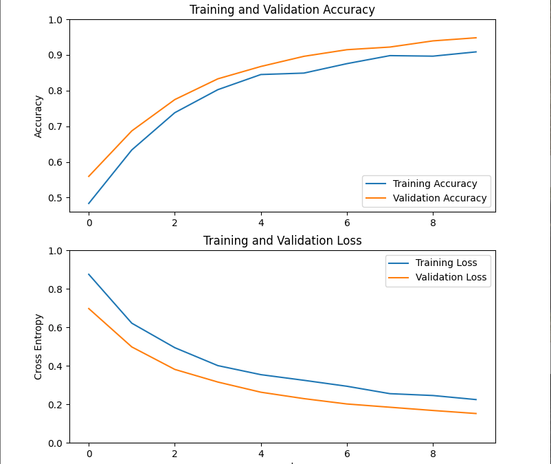
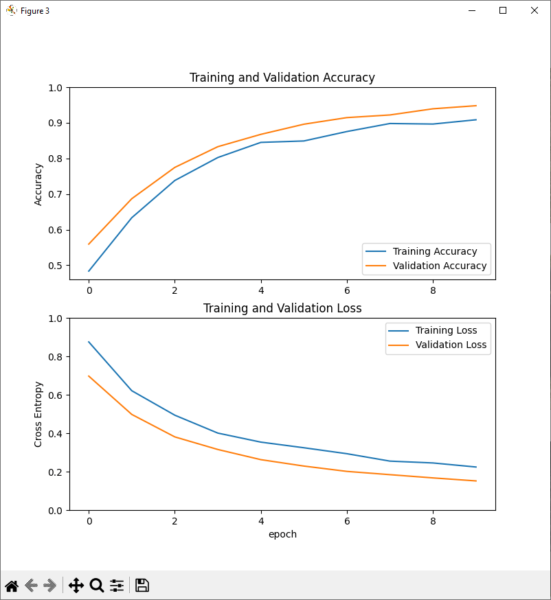
#plot learning curves
acc = history.history['accuracy']
val_acc = history.history['val_accuracy']
loss = history.history['loss']
val_loss = history.history['val_loss']
plt.figure(figsize=(8, 8))
plt.subplot(2, 1, 1)
plt.plot(acc, label='Training Accuracy')
plt.plot(val_acc, label='Validation Accuracy')
plt.legend(loc='lower right')
plt.ylabel('Accuracy')
plt.ylim([min(plt.ylim()),1])
plt.title('Training and Validation Accuracy')
plt.subplot(2, 1, 2)
plt.plot(loss, label='Training Loss')
plt.plot(val_loss, label='Validation Loss')
plt.legend(loc='upper right')
plt.ylabel('Cross Entropy')
plt.ylim([0,1.0])
plt.title('Training and Validation Loss')
plt.xlabel('epoch')
plt.show()
#fine tuning
base_model.trainable = True
# Let's take a look to see how many layers are in the base model
print("Number of layers in the base model: ", len(base_model.layers))
# Fine-tune from this layer onwards
fine_tune_at = 100
# Freeze all the layers before the `fine_tune_at` layer
for layer in base_model.layers[:fine_tune_at]:
layer.trainable = False
model.compile(loss=tf.keras.losses.BinaryCrossentropy(from_logits=True),
optimizer = tf.keras.optimizers.RMSprop(learning_rate=base_learning_rate/10),
metrics=['accuracy'])
model.summary()
fine_tune_epochs = 10
total_epochs = initial_epochs + fine_tune_epochs
history_fine = model.fit(train_dataset,
epochs=total_epochs,
initial_epoch=history.epoch[-1],
validation_data=validation_dataset)
#plot fine learning curves
acc += history_fine.history['accuracy']
val_acc += history_fine.history['val_accuracy']
loss += history_fine.history['loss']
val_loss += history_fine.history['val_loss']
plt.figure(figsize=(8, 8))
plt.subplot(2, 1, 1)
plt.plot(acc, label='Training Accuracy')
plt.plot(val_acc, label='Validation Accuracy')
plt.ylim([0.8, 1])
plt.plot([initial_epochs-1,initial_epochs-1],
plt.ylim(), label='Start Fine Tuning')
plt.legend(loc='lower right')
plt.title('Training and Validation Accuracy')
plt.subplot(2, 1, 2)
plt.plot(loss, label='Training Loss')
plt.plot(val_loss, label='Validation Loss')
plt.ylim([0, 1.0])
plt.plot([initial_epochs-1,initial_epochs-1],
plt.ylim(), label='Start Fine Tuning')
plt.legend(loc='upper right')
plt.title('Training and Validation Loss')
plt.xlabel('epoch')
plt.show()
#evaluate
loss, accuracy = model.evaluate(test_dataset)
print('Test accuracy :', accuracy)
model.save('saved_models/my_model')
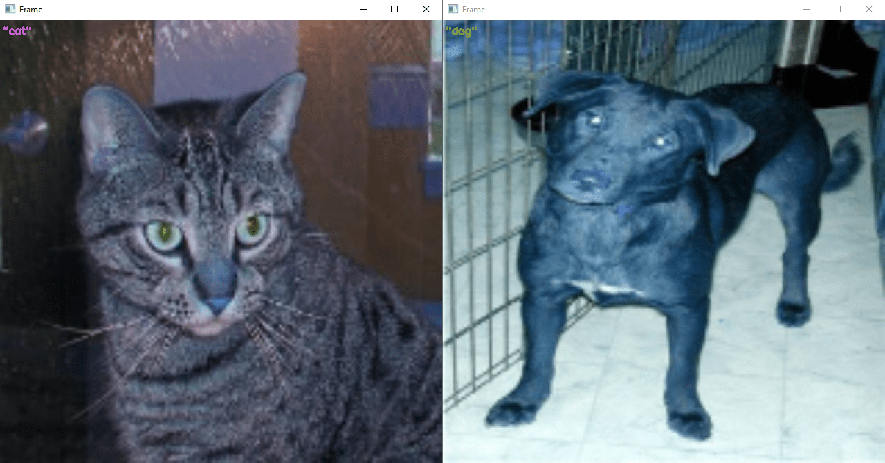
Utilisation du modèle entrainé
Vous pouvez utiliser le modèle entrainé pour classifier de nouvelles images contenant un seul type d’objet par image. Pour cela, il vous suffit de charger le modèle précédemment sauvegardé (saved_models/my_model)
#!/usr/bin/env python
# -*- coding: utf-8 -*-
#
#  ObjectRecognitionTFVideo.py
#  Description:
#		Use ModelNetV2-SSD model to detect objects on video
#
#  www.aranacorp.com

# import packages
import sys
from imutils.video import VideoStream
from imutils.video import FPS
import numpy as np
import argparse
import imutils
import time
import cv2
import tensorflow as tf
from PIL import Image

# load model from path
#model= tf.saved_model.load("./pretrained_models/ssd_mobilenet_v2_320x320_coco17_tpu-8/saved_model")
model= tf.saved_model.load("./saved_models/my_model")
#model.summary()

print("model loaded")

#load class names
#category_index = label_map_util.create_category_index_from_labelmap(PATH_TO_LABELS,use_display_name=True)
def read_label_map(label_map_path):

    item_id = None
    item_name = None
    items = {}

    with open(label_map_path, "r") as file:
        for line in file:
            line.replace(" ", "")
            if line == "item{":
                pass
            elif line == "}":
                pass
            elif "id" in line:
                item_id = int(line.split(":", 1)[1].strip())
            elif "display_name" in line: #elif "name" in line:
                item_name = line.split(":", 1)[1].replace("'", "").strip()

            if item_id is not None and item_name is not None:
                #items[item_name] = item_id
                items[item_id] = item_name
                item_id = None
                item_name = None

    return items

#class_names=read_label_map("./pretrained_models/ssd_mobilenet_v2_320x320_coco17_tpu-8/mscoco_label_map.pbtxt")
class_names = read_label_map("./saved_models/label_map.pbtxt")
class_names = list(class_names.values()) #convert to list
class_colors = np.random.uniform(0, 255, size=(len(class_names), 3))
print(class_names)

if __name__ == '__main__':

	# Open image
	#img= cv2.imread('./data/cats_and_dogs_filtered/train/cats/cat.1.jpg') #from image file
	img= cv2.imread('./data/cats_and_dogs_filtered/train/dogs/dog.1.jpg') #from image file
	img = cv2.resize(img,(160,160))
	img = cv2.cvtColor(img, cv2.COLOR_BGR2RGB)

	#input_tensor = np.expand_dims(img, 0)
	input_tensor = tf.convert_to_tensor(np.expand_dims(img, 0), dtype=tf.float32)

	# predict from model
	resp = model(input_tensor)
	print("resp: ",resp)
	score= tf.nn.sigmoid(resp).numpy()[0][0]*100
	cls = int(score>0.5)
	print("classId: ",int(cls))
	print("score: ",score)
	print("score: ",tf.nn.sigmoid(tf.nn.sigmoid(resp)))


	# write classname for bounding box
	cls=int(cls) #convert tensor to index
	label = "{}".format(class_names[cls])
	img = cv2.resize(img,(640,640))
	cv2.putText(img, label, (5, 20), cv2.FONT_HERSHEY_SIMPLEX, 0.5, class_colors[cls], 2)

	# Show frame
	cv2.imshow("Frame", img)
	cv2.waitKey(0)
Applications
- reconnaissance de différentes races d’animaux
- reconnaissance de différents type d’objets comme des cartes électroniques
Autres modèles de classification à considérer
- vgg16
- vgg19
- resnet50
- resnet101
- resnet152
- densenet121
- densenet169
- densenet201
- inceptionresnetv2
- inceptionv3
- mobilenet
- mobilenetv2
- nasnetlarge
- nasnetmobile
- xception